


Plankton and Primary Production
The phytoplankton of the ocean carry out close to half of all photosynthesis on Earth with less than one per cent of its photosynthetic biomass. This unit introduces the drifting life of the sea and the four groups of cells that do most of the work: diatoms, dinoflagellates, coccolithophores, and the cyanobacteria. It explains how light and nutrients set the limits of their growth, why the North Atlantic turns green each spring, and how primary production is measured from a bottle, a radioactive tracer, and a satellite.
Every second breath a person takes was made by cells they have never seen. The phytoplankton of the ocean, drifting algae and bacteria mostly smaller than the width of a hair, carry out close to half of all photosynthesis on Earth with less than 1 per cent of its photosynthetic biomass, and they manage this because they are eaten and replaced about once a week. This unit introduces the drifting life of the sea, the four groups of cells that do most of the work, the light and the nutrients that set their limits, the spring bloom that turns the North Atlantic green each year, and the methods by which all of this is measured, from a bottle on a rope to a satellite.
1 The drifting life
In 1887 the physiologist Victor Hensen (1835-1924), who worked in Kiel in northern Germany, needed a word for everything that is carried about by the water, and he chose the Greek word for “that which wanders”. Plankton is defined by its way of life, so a planktonic organism is one that cannot swim against a current, whatever its size. A jellyfish with a bell of a metre across is plankton, and so is a bacterium of less than a micrometre, whereas a sardine of 15 centimetres, which can hold its position against a current, is not. Animals that swim where they choose are the nekton, and organisms that live on or in the seabed are the benthos.
Within the plankton, the first division is by diet. The phytoplankton are the drifting photosynthesizers, algae and photosynthetic bacteria, and they are the subject of most of this unit. The zooplankton are the drifting animals and the animal-like single cells that eat other plankton. The bacterioplankton, the bacteria and archaea that do not photosynthesize but live on dissolved organic matter (biologists call such organisms heterotrophic), outnumber both, with about a million cells in every millilitre of seawater, and the viruses that infect them number some ten million in a millilitre; what the two do with the carbon that passes through them, the so-called microbial loop, goes beyond this unit.
Plankton is also divided by life history. The holoplankton spend their whole lives drifting, as copepods, krill, and most phytoplankton do, whereas the meroplankton, the eggs and larvae of crabs, barnacles, mussels, sea urchins, and most fishes, drift for weeks and then settle or swim away (Unit 4 returns to them). A third division is by size, and because plankton is sampled with nets and filters of a given mesh, the size classes of Table 1, proposed in 1978, are practical as well as descriptive.
| Size Class | Size Range | Typical Members |
|---|---|---|
| femtoplankton | 0.02 to 0.2 µm | viruses |
| picoplankton | 0.2 to 2 µm | bacteria, Prochlorococcus, Synechococcus |
| nanoplankton | 2 to 20 µm | coccolithophores, small flagellates, small diatoms |
| microplankton | 20 to 200 µm | most diatoms and dinoflagellates, ciliates |
| mesoplankton | 0.2 to 20 mm | copepods, fish eggs, most larvae |
| macroplankton | 2 to 20 cm | krill, arrow worms, small jellyfish |
| megaplankton | more than 20 cm | large jellyfish, salp chains, siphonophores |
Size decides almost everything else in the life of a drifting cell. A small cell has more surface for its volume, so it takes up scarce nutrients faster and sinks more slowly, which is why the smallest phytoplankton dominate the nutrient-poor open ocean; a large cell is harder for small grazers to eat and sinks faster when it dies, which is why the large diatoms dominate the rich waters of spring blooms and carry more carbon to depth.
2 The phytoplankton
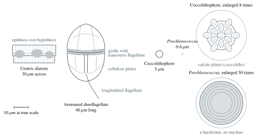
The phytoplankton is a collection of lineages from across the tree of life of Unit 1 that have each settled on the same way of living: a single cell, or a short chain of cells, that drifts in the sunlit layer, takes up dissolved nutrients through its surface, and fixes carbon by photosynthesis. Four groups do most of the work of the ocean, and a marine biologist recognizes each by its cell wall and its way of moving. Figure 1 draws one member of each at the same scale.
2.1 Diatoms
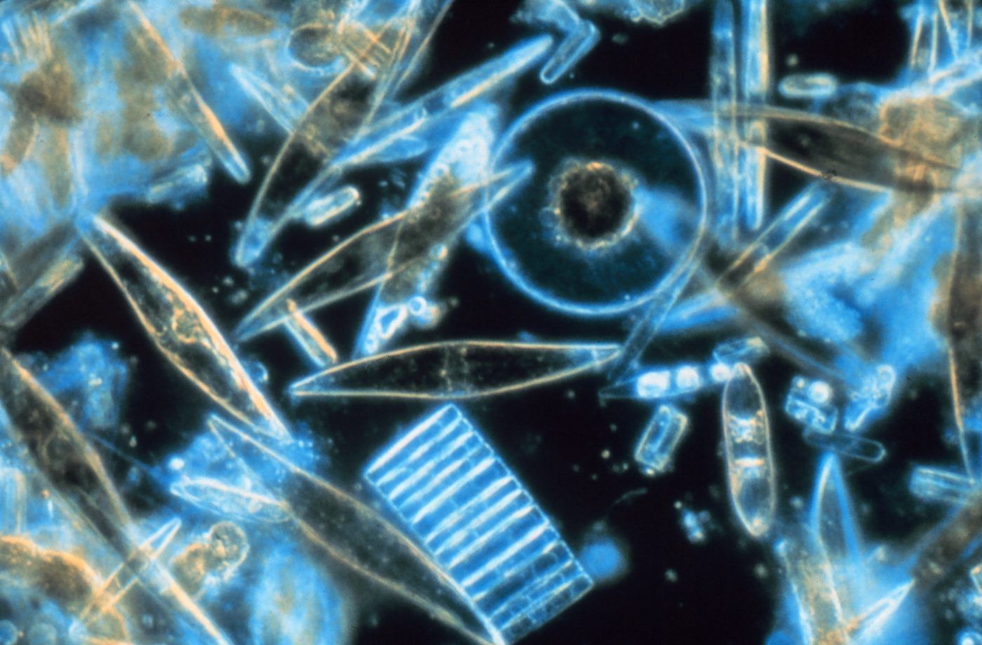
A diatom is a single-celled alga that lives inside a wall of glass. The wall, called the frustule, is made of hydrated silica, the material of opal, and consists of two valves that fit into each other like the two halves of a pill box or a Petri dish, the slightly larger valve, called the epitheca, over the slightly smaller one, called the hypotheca. The valves are perforated by a species-specific pattern of pores that lets dissolved gases and nutrients through. Diatoms come in two shapes, the round centric diatoms and the elongated pennate diatoms, and many species of both grow in chains (Figure 2). None of the planktonic ones can swim, although many pennate species of the seabed glide over surfaces. Most species are between 20 and 200 micrometres long, which makes them the largest of the four groups, and they dominate the spring blooms of temperate and polar seas, where they divide about once a day as long as light, nitrate, and dissolved silicon last. Because every diatom must take up silicon to build its wall, the amount of silicon the ocean’s diatoms use in a year gives an estimate of how much they grow; from this global silica budget, Nelson and colleagues estimated in 1995 that diatoms carry out roughly 40 per cent of all photosynthesis in the sea (the primary production of Section 6). Their glass walls make them heavy, so dead diatoms and chains sink fast, and the diatom blooms of spring are the main source of fresh organic matter for the deep seafloor, which Unit 8 follows downward.
2.2 Dinoflagellates
A dinoflagellate is a single cell with two flagella, whip-like threads used for swimming, of different form. One lies in a groove around the middle of the cell, the cingulum or girdle, and makes the cell spin; the other trails behind in a second groove, the sulcus, and drives the cell forward, so that a dinoflagellate swims in a spiral fast enough to move up and down by tens of metres in a day. Many species are armoured by plates of cellulose. About 2,000 living species are known, about half of them heterotrophic, living by eating other cells, and many of the photosynthetic ones also eat, a habit called mixotrophy. Dinoflagellates divide every few days rather than daily, and they take over in summer, when the water is stratified, with warm light water lying on cold dense water as Unit 2 described, and nutrients are scarce, because they can swim down at night to the nutrients and up in the morning to the light. A few species make the most dangerous substances in the plankton; for example, the saxitoxin of Alexandrium species accumulates in mussels and causes paralytic shellfish poisoning, so shellfish beds are closed when the cells are counted above a threshold. Dense blooms of some species colour the water brown or red, the origin of the old name red tide for any harmful bloom. The dinoflagellates of the family Symbiodiniaceae, long called zooxanthellae, live inside the cells of reef corals, which lie beyond this unit.
2.3 Coccolithophores
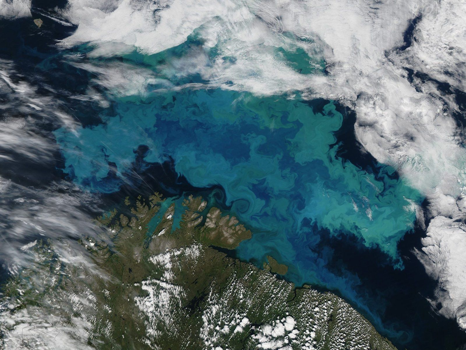
A coccolithophore is a small alga, mostly between 3 and 20 micrometres across, that covers itself with plates of calcium carbonate called coccoliths. The plates are made inside the cell in a species-specific shape and pushed out to the surface, where they overlap like roof tiles. Between 200 and 300 living species are known. The commonest by far is Gephyrocapsa huxleyi, which most of the literature still calls Emiliania huxleyi; genetic studies have placed it in the genus Gephyrocapsa, and both names are in use. It is about 5 micrometres across and blooms in late spring and summer in temperate and subpolar seas, after the diatoms have used up the dissolved silicon. When the cells die and shed their plates, the water fills with billions of tiny calcite mirrors that scatter sunlight back out of the sea, and the bloom turns the water a milky turquoise that is visible from orbit (Figure 3). Coccoliths that sink to the bottom accumulate over millions of years into chalk; the white cliffs of the English Channel are made of coccoliths that settled on the floor of a warm shelf sea in the Cretaceous period, between about 100 and 66 million years ago.
2.4 Cyanobacteria
The fourth group belongs to the bacteria rather than to the algae. Cyanobacteria are the bacteria that photosynthesize with chlorophyll and release oxygen, as plants do, and two genera of them dominate the picoplankton of the warm ocean. Synechococcus, a cell of about 1 micrometre, was recognized as a major component of the open ocean in 1979. Prochlorococcus, with cells of 0.5 to 0.7 micrometres, was discovered only in 1988 by Sallie Chisholm and her colleagues, who found it with a flow cytometer, the laser cell counter of Unit 1, because the cells were too small and dim for a microscope. A global count from more than 35,000 samples, published by Flombaum and colleagues in 2013, gave about \(3\times10^{27}\) Prochlorococcus cells in the ocean, a 3 followed by 27 zeros and far more than there are grains of sand on Earth, and about \(7\times10^{26}\) Synechococcus cells, and together the two genera are estimated to carry out about a quarter of all marine photosynthesis. Prochlorococcus lives in the warm belt between about 40 degrees north and south, and its whole strategy is its size, because the surface of a sphere grows with the square of its diameter and its volume with the cube, so the surface per unit of volume is inversely proportional to the diameter, and a sphere of 0.6 micrometres therefore has \(30/0.6 = 50\) times more surface for its volume than a diatom of 30 micrometres. It can therefore live on nutrient concentrations that would starve any larger cell.
The four groups divide the ocean by this logic. The fast-growing, heavy diatoms win where nutrients arrive in pulses, as in the spring of temperate seas and in upwelling regions. The tiny cyanobacteria win where the water is permanently stratified and poor, and dinoflagellates and coccolithophores take the seasons in between. Section 4 explains what sets the supply.
3 Light and photosynthesis in the sea
A phytoplankton cell gains carbon by photosynthesis and loses it by respiration, and both rates can be measured. Photosynthesis depends on light, which Unit 2 showed to fade exponentially with depth according to the Beer-Lambert law, \(E(z) = E_0\,e^{-K_d z}\), with \(E_0\) the irradiance just below the surface and \(K_d\) the attenuation coefficient. The quantity that matters to the cell is the photosynthetically active radiation, or PAR, the light between 400 and 700 nanometres that chlorophyll and its helper pigments can absorb, counted as photons arriving on a square metre each second, in \(\mathrm{\mu mol\,photons\,m^{-2}\,s^{-1}}\). A micromole of photons is about \(6\times10^{17}\) of them, and full sunlight at noon delivers about \(2{,}000\unit{\mu mol\,photons\,m^{-2}\,s^{-1}}\) to the sea surface. When the light of a whole day is added up, it is given in moles of photons per square metre per day instead; one mole per day is about 12 micromoles per second averaged over the 24 hours, and a clear summer day delivers a few tens of moles to each square metre of sea. Both units appear in this section, the first for measurements that take minutes, the second for the balance of a day.
3.1 The photosynthesis-irradiance curve
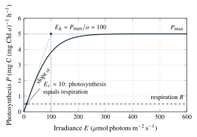
When the photosynthesis of a sample of phytoplankton is measured at a series of light levels, the result is the photosynthesis-irradiance curve, usually called the P-I curve, and Figure 4 shows its form. At low light the rate rises in proportion to the light, because every photon absorbed is used, and the slope of this part, written \(\alpha\), measures how efficiently the cells use dim light. At high light the rate levels off at a maximum, \(P_{\max}\), because the enzymes that fix carbon are working as fast as they can and additional photons are wasted. The irradiance at which the initial slope, if continued, would reach the maximum is the saturation irradiance \(E_k = P_{\max}/\alpha\). In very bright light the curve often turns down again, because the light damages the photosynthetic machinery faster than the cell can repair it, which is called photoinhibition.
3.2 Compensation depth and critical depth
Light is a function of depth, so the P-I curve can be read as a profile, that is, as a plot of the photosynthesis rate against depth. Respiration, by contrast, hardly depends on light, and to a first approximation a cell respires at the same rate at every depth, day and night. There is therefore an irradiance at which photosynthesis equals respiration, the compensation irradiance \(E_c\), and a depth at which the light has fallen to that value, the compensation depth \(z_c\). A cell above the compensation depth gains carbon over a day; a cell below it loses carbon and will, in time, starve. Textbooks often place it close to the 1 per cent light depth, the bottom of the euphotic zone of Unit 2, but the compensation irradiance measured for different species and communities varies by a factor of ten, and the depth varies with it.
A cell in the ocean does not sit still. In winter, storms and the cooling of the surface mix the upper water column to depths of a hundred metres and more, and a phytoplankton cell is carried through the whole of the mixed layer, spending part of its time in the light near the surface and part in the dark far below the compensation depth, so what matters for it is the balance over the whole layer. The Norwegian oceanographer Harald Sverdrup (1888-1957), who had led the Scripps Institution of Oceanography in California for twelve years before returning to Norway, put this into a clear criterion in 1953, using measurements from a weather ship in the Norwegian Sea.
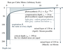
In Figure 5 the critical depth is far deeper than the compensation depth, because the surplus gained in the bright water near the surface pays for a long stretch of slight losses below; the following mechanism turns the picture into a formula.
3.3 The North Atlantic spring bloom and what starts it
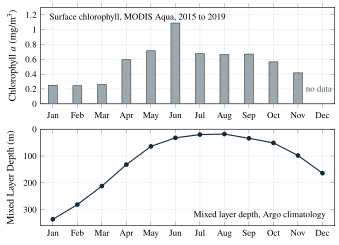
Each spring, the North Atlantic between about 40 and 65 degrees north turns from blue to green over a few weeks, one of the largest seasonal events of the living ocean and the subject of the picture at the head of this unit. In winter the mixed layer of its subpolar part is 200 to 400 metres deep and the surface chlorophyll is low, around \(0.2\unit{mg\,m^{-3}}\). From April onward the surface warms, the mixed layer shrinks to tens of metres, and the chlorophyll rises within a month to several milligrams per cubic metre as diatoms divide once a day on the nitrate, phosphate, and silicate that the winter mixing brought up from below. By June the silicate and then the nitrate of the surface layer are used up, the diatoms sink or are eaten, and the bloom ends as quickly as it began. Figure 6 shows this cycle in the monthly means at one site in the eastern North Atlantic.
Sverdrup’s model was the accepted explanation of the spring bloom for half a century, and the satellite record then raised a difficulty. When Michael Behrenfeld examined nine years of SeaWiFS data for the subarctic Atlantic in 2010, he found that the total amount of phytoplankton under a square metre begins to increase in midwinter, when the mixed layer is still deepening and far deeper than any critical depth. His explanation, first called the dilution-recoupling hypothesis and later the disturbance-recovery hypothesis, moves the attention from the plants to their predators. A bloom, in this view, is any period in which the division rate of the phytoplankton exceeds their loss rate, which is mostly grazing. When winter mixing dilutes the plankton, the grazers meet their prey less often and the balance tips in favour of the phytoplankton, even though light and division rate are at their lowest; in spring the division rate accelerates and stays ahead of the grazers for a while, which is the visible bloom, until the grazers catch up. The dispute is not settled, and the research spotlight describes the field programme designed to settle it.
4 Nutrients and what limits growth
Light decides where photosynthesis can take place, and the supply of nutrients decides how much of it there is. A phytoplankton cell builds itself from carbon, which seawater holds in abundance as dissolved carbon dioxide and bicarbonate, and from elements that seawater holds in short supply. The three that run out first are nitrogen, taken up mostly as nitrate (\(\mathrm{NO_3^-}\)) and ammonium (\(\mathrm{NH_4^+}\)), phosphorus as phosphate (\(\mathrm{PO_4^{3-}}\)), and, for diatoms only, silicon as dissolved silicic acid, called silicate. Behind these comes iron, which the enzymes of photosynthesis and of nitrate uptake need in tiny amounts. Surface water in the subtropical gyres holds nitrate below \(0.1\unit{\mu mol\,L^{-1}}\), whereas the deep water below a thousand metres holds some 20 to \(40\unit{\mu mol\,L^{-1}}\), because that is where the sinking remains of the plankton are decomposed. How fast this deep store returns to the light, by winter mixing and by the upwelling of Unit 2, sets the productivity of the sea.
4.1 The Redfield ratio
In 1934 Alfred Redfield (1890-1983) of the Woods Hole Oceanographic Institution noticed that the ratio of nitrate to phosphate in deep seawater from every ocean was nearly constant, about 20 atoms of nitrogen for every atom of phosphorus by his first estimate, and that the plankton collected at the surface had, on average, the same ratio in their tissues. He concluded that the composition of the deep water is set by the decay of the plankton. Richard Fleming revised the plankton analyses to 16 atoms of nitrogen per atom of phosphorus and added carbon in 1940, and Redfield gave the ratio its modern form in 1958.
4.2 Liebig’s law and the limiting nutrient
Which nutrient runs out first is decided by a principle from agricultural chemistry. In 1840 Justus von Liebig (1803-1873) stated, building on the soil studies of Carl Sprengel (1787-1859), that the yield of a crop is set by the nutrient that is scarcest in relation to the plant’s needs and not by the total amount of all nutrients.
Over most of the low-latitude ocean the limiting nutrient is nitrogen, because the ratio of nitrate to phosphate in the surface water is a little below 16 and because nitrogen is lost from the sea by bacteria that turn nitrate back into nitrogen gas, a cycle that goes beyond this unit. For diatoms the first nutrient to run out in spring is often silicate, which is why diatom blooms end before the nitrate is gone and hand over to groups that need no silica, such as the coccolithophores. The most surprising case concerns the three regions where nitrate and phosphate remain high all year and the phytoplankton still fail to grow, the Southern Ocean, the equatorial Pacific, and the subarctic North Pacific, together roughly a quarter of the ocean’s surface, known as the high-nutrient, low-chlorophyll regions. The missing element there is iron, which reaches the open sea mainly as dust blown from deserts, and these three regions lie far from any desert.
5 The grazers
More than half of what the phytoplankton produce is eaten within a few days. Measured over the whole ocean, the greater part of it, about two thirds, goes to single-celled grazers of the microplankton, the ciliates, which are cells that swim and feed with rows of tiny hairs, and the heterotrophic dinoflagellates, and both divide as fast as their prey; the rest goes to three groups of animals. The copepods are small crustaceans, most of them 1 to 5 millimetres long, that filter or catch single phytoplankton cells with their feeding limbs, and they are probably the most numerous animals on Earth. For example, Calanus finmarchicus, a copepod of 2 to 4 millimetres, is the main grazer of the North Atlantic spring bloom and the main food of herring, mackerel, and the right whale. The krill are shrimp-like crustaceans of a few centimetres; the Antarctic krill (Euphausia superba) forms swarms of thousands of animals per cubic metre and has a total biomass of a few hundred million tonnes (379 million tonnes in the most cited estimate, by Atkinson and colleagues in 2009), which is about the combined weight of all the people on Earth, and this biomass feeds the whales, seals, and penguins of the Southern Ocean. The gelatinous zooplankton, the jellyfish, comb jellies, and salps, are mostly water, multiply fast when food is plentiful, and pack what they filter into dense faecal pellets that sink hundreds of metres a day. Unit 4 describes the anatomy of these animals, and the fate of the pellets and the uneaten cells, the biological pump that carries carbon to the deep sea, is the subject of Unit 8.
6 Measuring production and the global picture
6.1 Three ways to measure primary production
Primary production is the rate at which the phytoplankton fix carbon by photosynthesis, measured in milligrams of carbon per cubic metre per day or, summed over the sunlit layer, per square metre per day or per year. Gross primary production is the total carbon fixed, net primary production is what remains after the respiration of the phytoplankton themselves, and only the second is available to the rest of the food web. Three methods measure it, the oldest with bottles and dissolved oxygen, the second with a radioactive tracer, and the third from orbit.
The oldest method, introduced in 1927 by the Norwegian scientists Torbjørn Gaarder and Haaken Hasberg Gran, uses pairs of glass bottles filled with seawater and its plankton and hung at a series of depths for a day. In the clear bottle the oxygen rises by photosynthesis and falls by respiration; in the bottle painted black it can only fall. The dark bottle therefore gives the respiration, the light bottle the net production, and their sum the gross production, all in oxygen, which is converted into carbon with the photosynthetic quotient, the moles of oxygen released per mole of carbon fixed, between about 1.0 and 1.4 depending on whether the cells grow on ammonium or on nitrate, because a cell that takes up nitrate must first reduce it and releases extra oxygen in doing so.
The method that made the global map possible came in 1952 from the Danish botanist Einer Steemann Nielsen (1907-1989) on the Danish Galathea expedition round the world. A small amount of bicarbonate labelled with the radioactive isotope carbon-14 is added to a bottle of seawater, the bottle is incubated in the light, and at the end the cells are filtered out and their radioactivity is measured. Because the labelled carbon mixes evenly with the ordinary dissolved carbon, the cells take up the same fraction of both, so the fraction of the added label found in the cells, multiplied by the dissolved inorganic carbon of the water, is the carbon fixed. The method detects production about a hundred times smaller than the oxygen bottles can and is the standard against which the others are calibrated; its weaknesses are that the result lies between gross and net production, because some labelled carbon is respired again during the incubation, and that a bottle is a cage, in which the community changes during a long incubation.
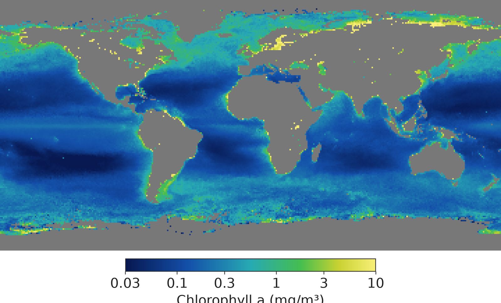
The third method does not touch the water. Chlorophyll \(a\) absorbs blue and red light and leaves the green, so the colour of the sea, measured from orbit, gives the concentration of chlorophyll in the uppermost layer, roughly the top \(1/K_d\) metres, which is a few tens of metres in clear water and a few metres in turbid water. The first instrument to do this was the Coastal Zone Color Scanner on the Nimbus-7 satellite, from 1978 to 1986, followed by SeaWiFS from 1997 to 2010, MODIS on the Aqua satellite since 2002, and the PACE mission launched in 2024. A satellite sees the whole ocean every few days, and Figure 7 shows a year of its view. The step from chlorophyll to production needs a model built on the P-I curve, the light, the temperature, and the depth of the sunlit layer, calibrated against thousands of carbon-14 measurements. The leading models agree on the global total to within about 20 per cent, but a comparison of two dozen models by Carr and colleagues in 2006 found totals that differed by a factor of two, so the number is less certain than the map suggests.
6.2 The global numbers
Figure 7 answers one of the opening questions by inspection. The clearest and bluest water of the ocean, in the five subtropical gyres, holds the least chlorophyll, below \(0.1\unit{mg\,m^{-3}}\), because the water there is warm and permanently stratified, so that the nutrients released in the deep are never mixed back to the light. The coasts, the upwelling regions, and the high latitudes hold ten to a hundred times more, because rivers, upwelling, or winter mixing supply nutrients there.
Summed over the ocean, the satellite models give a net primary production of about \(50\unit{Pg\,C}\) per year, where one petagram is \(10^{15}\) grams, a billion tonnes, also written as one gigatonne. The most cited estimate, by Field and colleagues in 1998, was 48.5 petagrams of carbon for the ocean against 104.9 for the whole planet, so the sea fixes close to half of the carbon fixed on Earth each year. Spread over the 361 million square kilometres of the ocean, the average is about \(140\unit{g\,C\,m^{-2}\,yr^{-1}}\), below 50 in the gyres and above 300 in the upwelling regions and the shelf seas. The key result below sums this up, and the example compares it with the land.
The seasonal cycle behind the map differs with latitude in a way that follows from everything in this unit. In temperate and subpolar seas winter mixing recharges the nutrients, the spring bloom follows the shallowing of the mixed layer, and the first autumn storms often mix enough nutrient into still well-lit water for a second, smaller bloom. In polar seas light is the stronger limit, and there is a single short bloom in summer, often at the edge of the retreating sea ice, where melt water forms a shallow, stable layer. In the tropics and subtropics the water is stratified all year and the surface chlorophyll stays low and nearly constant. The largest concentration of cells there sits in a thin layer near the bottom of the sunlit zone, where light from above and nutrients from below just overlap, and this layer is called the deep chlorophyll maximum. The upwelling regions, where the seasons follow the winds rather than the sun, are the exception.